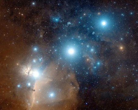
Strehl ratio
A measure of optical quality relative to a perfect system.

ESO · CC BY 4.0
The Strehl ratio, named after its proposer Karl Strehl, quantifies how well an optical system forms an image. It ranges from 0 to 1, where 1 represents a hypothetical perfect system free of aberrations. This metric applies when resolution is degraded by lens flaws or atmospheric turbulence.
Mathematically, the Strehl ratio \( S \) is often defined as the peak intensity of an aberrated point-source image divided by the maximum possible intensity from a diffraction-limited ideal system using the same aperture. Alternatively, it can be defined using the intensity at the image center for an on-axis source; in most practical cases, these definitions yield nearly identical values, especially when symmetry forces the peak to lie at the center. With the latter definition, \( S \) is computed from the wavefront error \( \delta(x,y) \), which is the deviation of the actual wavefront from an ideal one over the aperture \( A(x,y) \). Using Fraunhofer diffraction, the wave amplitude at the image center is found via the Fourier transform of the aberrated pupil function, where phase factors reduce to unity.
\[ S = |\langle e^{i\phi} \rangle|^2 = |\langle e^{i2\pi \delta / \lambda} \rangle|^2 \]
Here, \( i \) is the imaginary unit, \( \phi = 2\pi \delta / \lambda \) is the phase error at wavelength \( \lambda \), and the angle brackets denote an average over the aperture.
\[ S \approx e^{-\sigma^2} \]
where \( \sigma^2 = \langle (\phi - \bar{\phi})^2 \rangle \) is the variance of the phase over the aperture.
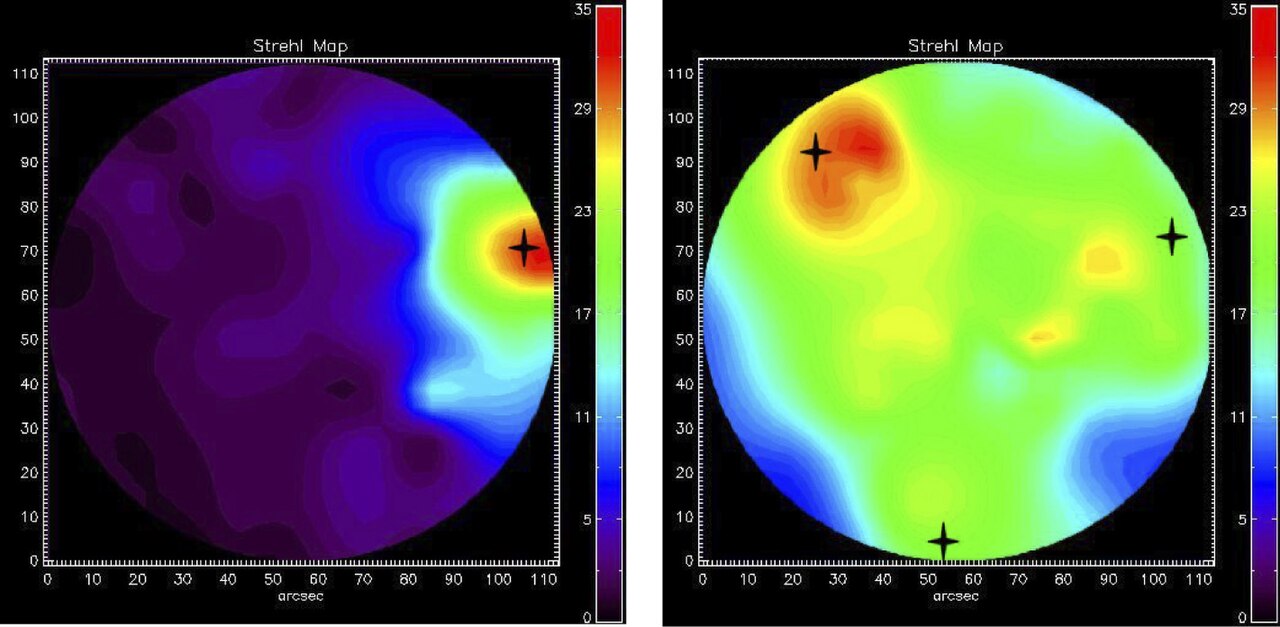
Even a geometrically perfect focusing system is limited by diffraction. For a uniform circular aperture, the point spread function (PSF) of a point source is the Airy disk. The peak intensity at the center of this Airy disk defines the reference for a Strehl ratio of 1. An imperfect system using the same aperture typically produces a broader PSF with a lower peak, reduced by the Strehl ratio. Systems with only minor imperfections are called "diffraction limited" if their PSF closely matches the Airy disk; a Strehl ratio above 0.8 is often used as the threshold for this designation.
- Proposed by
- Karl Strehl
- Value range
- 0 to 1
- Perfect system value
- 1
- Diffraction limited threshold
- greater than 0.8
- Mathematical approximation
- S ≈ e^(-σ²)
- Wavelength dependence
- peak intensity falls as λ⁻²
Lore & Background
The Strehl ratio is frequently defined as the ratio of the peak aberrated image intensity from a point source compared to the maximum attainable intensity using an ideal optical system limited only by diffraction over the system's aperture. It can also be expressed in terms of the intensity at the image center due to an on-axis source; in most important cases these definitions result in a very similar or identical figure. Using Fraunhofer diffraction theory, the Strehl ratio is computed from the squared magnitude of the wave amplitude, given by S = |⟨e^(iϕ)⟩|², where ϕ is the phase error over the aperture at wavelength λ. The ratio can be estimated using only the statistics of the phase deviation via the Ruze formula, S ≈ e^(-σ²), where σ is the root mean square deviation of the wavefront phase.
Due to diffraction, even a perfect focusing system has limited spatial resolution, described by the Airy disk for a uniform circular aperture. An imperfect system produces a broader point spread function (PSF) with reduced peak intensity according to the Strehl ratio. An optical system with only minor imperfections may be called 'diffraction limited' if its PSF closely resembles the Airy disk; a Strehl ratio greater than 0.8 is frequently cited as the criterion for that designation. The size of the Airy disk grows linearly with wavelength, and the peak intensity falls as λ⁻², so the reference point for unity Strehl ratio changes; typically, longer wavelengths yield a better Strehl ratio even though actual image resolution is poorer.
Reader's Guide
The Strehl ratio is commonly used to assess the quality of astronomical seeing in the presence of atmospheric turbulence and to evaluate the performance of adaptive optical correction systems. It is also used for selecting short exposure images in the lucky imaging method. In industry, the Strehl ratio has become a popular way to summarize the performance of an optical design because it compares a real system, of finite cost and complexity, to a theoretically perfect system that would be infinitely expensive and complex to build. It provides a simple method to decide whether a system with a Strehl ratio of, for example, 0.95 is good enough, or whether twice as much should be spent to achieve a ratio of perhaps 0.97 or 0.98.
Characterizing the point-spread function by a single number is meaningful only if the PSF is little distorted from its ideal form, which is true for well-corrected systems operating near the diffraction limit, including most telescopes and microscopes, but excluding most photographic systems. The Strehl ratio has been linked via the work of André Maréchal to an aberration tolerancing theory useful to designers of well-corrected optical systems, allowing a meaningful link between geometrical optics aberrations and diffraction theory. A significant shortcoming is that, although relatively easy to calculate for an optical design on paper, it is normally difficult to measure for a real optical system, not least because the theoretical maximum peak intensity is not readily available.
Did You Know?
- The Strehl ratio was originally proposed by Karl Strehl, after whom the term is named.
- The Strehl ratio is difficult to measure for a real optical system because the theoretical maximum peak intensity is not readily available.
The Core Mechanism: Capturing Fleeting Clarity
Lucky imaging operates on a deceptively simple premise: the Earth's atmosphere distorts starlight in constantly shifting patterns, producing the familiar twinkle visible to the naked eye. Rather than fighting this turbulence with a single long exposure that averages all the distortion, the technique uses a high-speed camera to capture thousands of extremely short frames, each lasting 100 milliseconds or less. During such a brief window, atmospheric changes are minimal, and a small fraction of frames—often around ten percent, or even just one percent in the most demanding applications—will be nearly free of distortion. These select frames are then aligned and summed together. The result is a composite image whose angular resolution can exceed that of a conventional long exposure by a factor of at least five, pushing even a 2.5-meter ground-based telescope to its theoretical diffraction limit. The stronger the selection criterion, the more the surrounding seeing halo is suppressed and the signal-to-noise ratio of point sources improves.
Three Decades of Refinement
The roots of lucky imaging stretch back to the middle of the twentieth century, when astronomers first began capturing planetary images with cine cameras and image intensifiers during the 1950s and 1960s. However, the technique remained impractical for roughly three decades while the separate imaging technologies needed for it were gradually perfected. A landmark moment came in 1978, when David L. Fried published the first numerical calculation of the probability of obtaining a genuinely lucky exposure. Early practitioners assumed the atmosphere simply smeared or blurred the image, so they estimated the full width at half maximum of that blur to pick the best frames. A later, more sophisticated understanding revealed that the atmosphere actually produces multiple sharp speckled copies of the source rather than a single smeared blob, and methods exploiting this speckle structure yielded dramatically superior results. By the early 2000s, researchers further recognized that turbulent intermittency—the natural fluctuation in seeing conditions—could substantially boost the odds of capturing a lucky frame for any given average atmospheric state.
Marrying Lucky Imaging with Adaptive Optics
In 2007, teams from Caltech and the University of Cambridge announced the first successful results from a hybrid system that combined lucky imaging with adaptive optics. Tested on the 200-inch Hale Telescope at Mount Palomar, the setup achieved diffraction-limited resolution in visible light on a five-meter-class instrument for the first time, reaching angular resolutions as fine as 0.025 arcseconds for certain observations. The logic is elegant: the lucky imaging camera identifies the brief sub-second intervals when atmospheric turbulence is mild enough that the adaptive optics correction alone can deliver excellent sharpness. Only those privileged frames are averaged into the final image. The approach does carry constraints, though. The crisp field of view is narrow, typically ten to twenty arcseconds, and the technique works best on targets no larger than ten arcseconds across. A relatively bright guide star of around fourteenth magnitude must also sit within the field. Airglow and the atmosphere's absorption of certain electromagnetic frequencies remain limitations that a space-based platform like the 2.4-meter Hubble simply does not face.
From Professional Observatories to Backyard Telescopes
What began as a specialized professional technique has become accessible to amateur astronomers as well, largely thanks to the proliferation of sensitive webcams and camcorders capable of recording rapid short exposures. When a user captures a video sequence through a telescope, discards the poorest frames, and stacks the remainder using the shift-and-add method inherited from speckle imaging, the result is effectively lucky imaging. Several distinct selection algorithms exist for picking the best frames. The Strehl-selection method, first proposed by John E. Baldwin of the Cambridge group, evaluates each frame's quality using the Strehl ratio as a figure of merit. An alternative approach, the Selective Image Reconstruction method developed by Ron Dantowitz, relies on image contrast as the selection criterion. In a notable demonstration, fifty thousand frames captured at nearly forty per second from the Calar Alto 2.2-meter telescope were processed to reveal a triple star system at roughly 45 parsecs, with the two faintest components separated by less than 0.16 arcseconds—equivalent to about 7.2 astronomical units, or one billion kilometers—confirming that the telescope had reached its diffraction limit.
Gallery
Frequently Asked Questions
Who came up with the Strehl ratio?
The metric is named after Karl Strehl, who proposed it as a way to quantify how closely an optical system approaches ideal image formation.
What does a Strehl ratio of 1 actually mean?
A value of 1 corresponds to a hypothetical system with zero aberrations, where the peak intensity of a point-source image equals the theoretical diffraction-limited maximum for that aperture.
What Strehl ratio counts as diffraction-limited?
A ratio above 0.8 is the commonly cited threshold for calling a system diffraction-limited, meaning wavefront errors from the optics or atmosphere are small enough that the image is near the theoretical best.
How do you estimate Strehl ratio from wavefront error?
For small aberrations the ratio is approximated as S ≈ e^(−σ²), where σ is the root-mean-square wavefront deviation expressed in radians.
Why does Strehl ratio matter in astrophotography?
It gives you a single number that captures how much lens flaws or atmospheric turbulence are degrading your star images relative to the perfect-case limit, making it a handy benchmark for comparing telescopes, seeing conditions, or adaptive-optics performance.
More in Astrophotography, Part 2 1-24
Spotted an error? Know more?
Reader corrections go straight into our review queue. Suggest an edit · How this site is sourced