
Poisson distribution
Discrete distribution for rare events in fixed intervals.

Sergio01 · CC BY-SA 3.0
The Poisson distribution is a discrete probability distribution used in probability theory and statistics. It calculates the likelihood of a specific number of events happening within a fixed interval—such as time, area, or volume—provided the events occur at a known constant average rate and independently of when the last event happened. This distribution is named after the French mathematician Siméon Denis Poisson.
For example, if a call center averages 3 calls per minute, and the number of calls in any two separate time intervals is independent, then the number of calls in a given minute follows a Poisson distribution. The probability of receiving exactly 3 calls is about 0.77, while the chance of receiving 0 or at least 5 calls is roughly 0.23. A classic motivating example is the count of radioactive decay events over a fixed observation period.
The Poisson distribution was introduced by Siméon Denis Poisson (1781–1840) in his 1837 work *Recherches sur la probabilité des jugements en matière criminelle et en matière civile*, which examined wrongful convictions by counting events over a time interval. However, Abraham de Moivre had already produced similar results in 1711 in *De Mensura Sortis seu; de Probabilitate Eventuum in Ludis a Casu Fortuito Pendentibus*. This makes it an instance of Stigler's law, leading some to argue the distribution should be named after de Moivre. In 1860, Simon Newcomb applied the Poisson distribution to the number of stars in a unit of space. Later, in 1898, Ladislaus Bortkiewicz showed that the frequency of Prussian soldiers accidentally killed by horse kicks fit the distribution well.
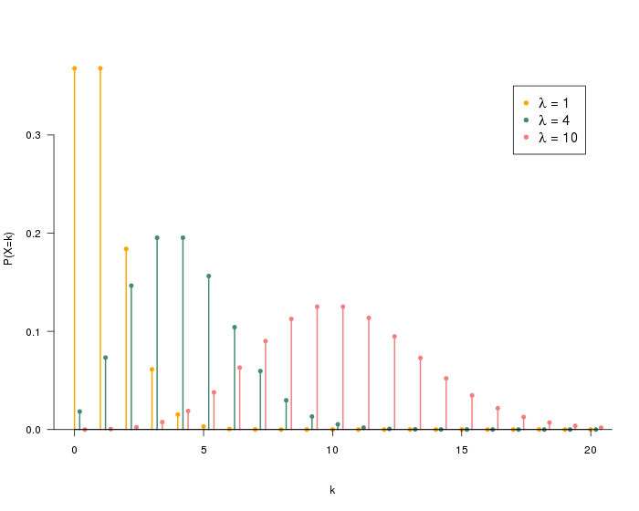
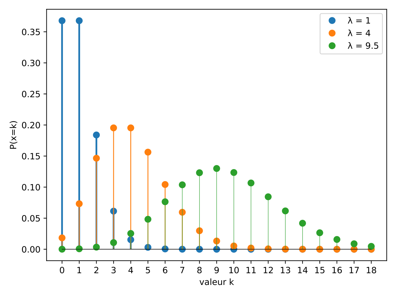
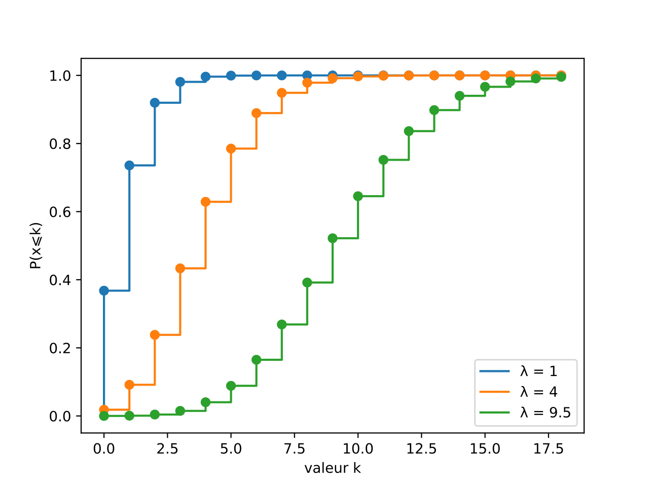
A discrete random variable \(X\) has a Poisson distribution with parameter \(\lambda\) if its probability mass function is: \[ P(X = k) = \frac{e^{-\lambda} \lambda^k}{k!} \] where \(k\) is the number of occurrences (a nonnegative integer), \(e\) is Euler's number, and \(k!\) is the factorial. The parameter \(\lambda\) is a positive real number equal to both the expected value and the variance of \(X\). This distribution is useful for systems with many possible events, each rare, under the right conditions. If the average rate \(r\) is given instead of the average number \(\lambda\), then \(\lambda = rt\), where \(t\) is the interval length.
The Poisson distribution can model events like the number of meteorites over one meter in diameter striking Earth in a year, laser photons hitting a detector in a specific time interval, students achieving low or high marks on an exam, or locations of defects and dislocations in materials. Random points in space, such as asteroid impacts on Earth (2-dimensional), material imperfections (3-dimensional), or tree locations in a forest (2-dimensional), also follow this distribution.
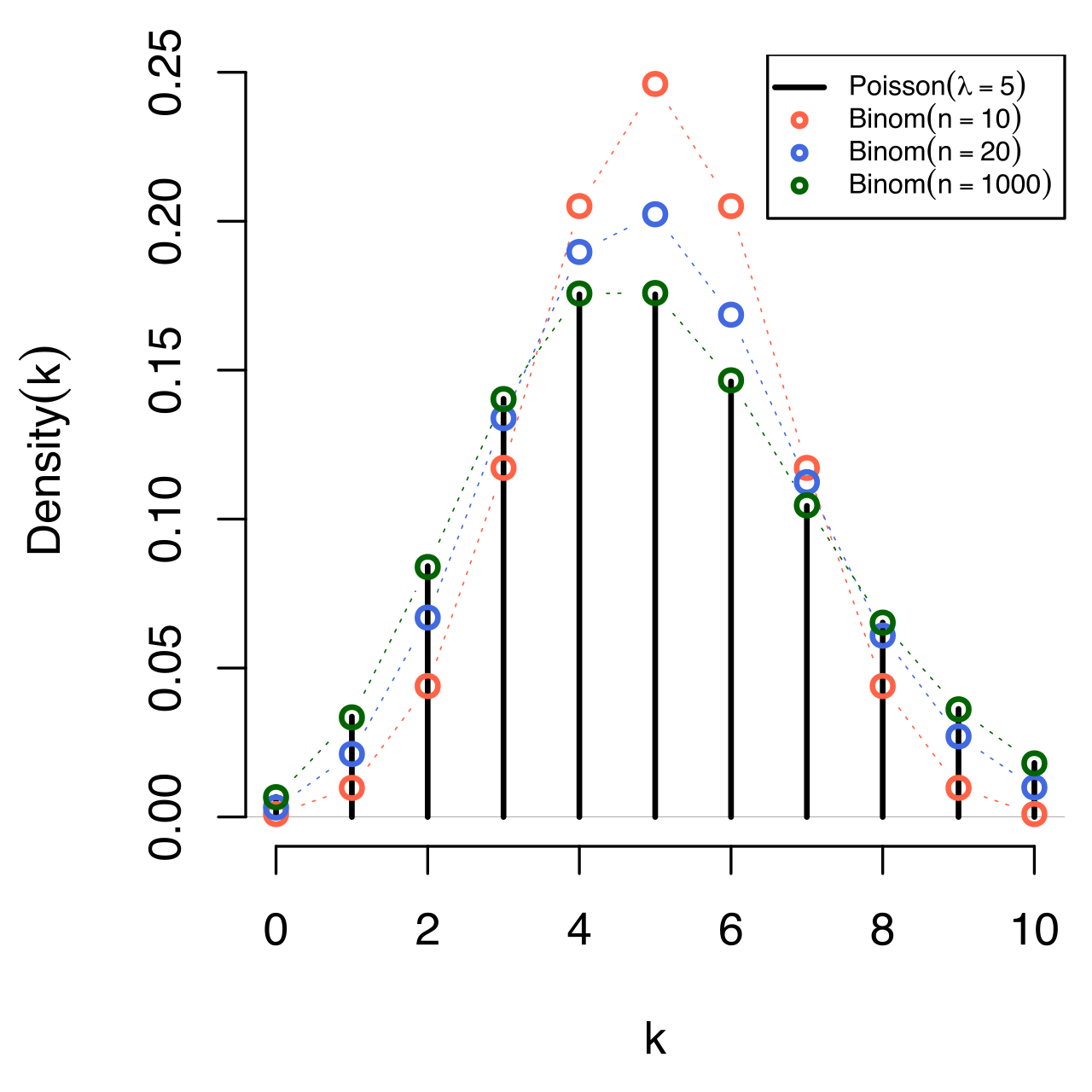
For the Poisson model to be appropriate, these assumptions must hold: \(k\) (a nonnegative integer) is the count of events in an interval; one event does not affect the probability of another; the average event rate is independent of any occurrences; and two events cannot happen at exactly the same instant. If these conditions are met, \(k\) is a Poisson random variable. The Poisson distribution is also the limit of a binomial distribution as the number of trials \(n\) goes to infinity while the expectation \(\lambda\) stays constant, with the probability of success per trial being \(\lambda/n\). It can also be derived from differential equations with initial conditions.
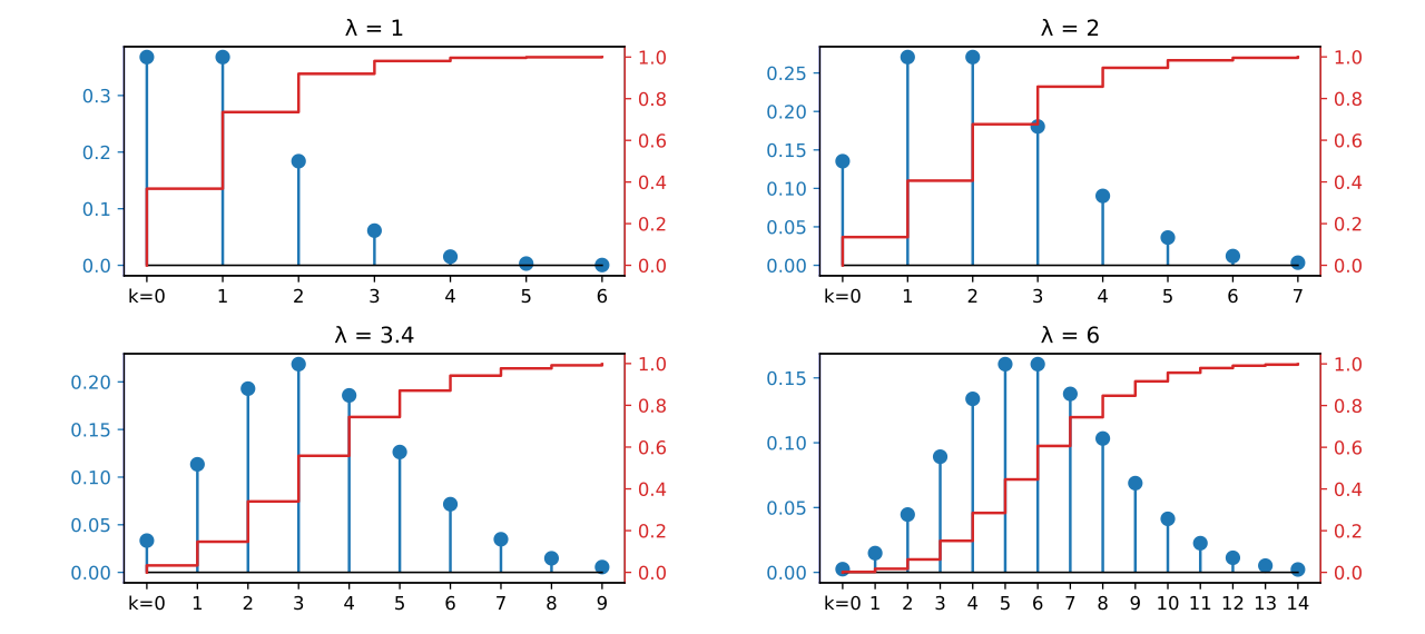
As an example, if a river overflows once every 100 years on average, the probability of 0 to 6 floods in a 100-year interval can be calculated using \(\lambda = 1\). For a World Cup soccer match with an average of 2.5 goals, the probability of 0 to 7 goals per match can be found similarly. However, the number of students arriving at a student union per minute likely violates the assumptions, as the rate is not constant (low during class, high between classes) and arrivals are not independent (students often come in groups). Such cases can be modeled with a mixed Poisson distribution or a compound Poisson process.
- field
- Probability theory and statistics
- known_for
- Poisson distribution
Quick Facts
- Notation
- \operatorname{Pois}(\lambda)
- Parameters
- \lambda\in (0, \infty) / (rate)
- Support
- k \in \mathbb{N}_0 / (Natural numbers starting from 0)
- \frac{\lambda^{k}e^{-\lambda
Facts from the source article.
Lore & Background
The Poisson distribution is a discrete probability distribution used to model the number of events occurring within a fixed interval of time, area, or volume, given that these events happen at a known constant mean rate and independently of the time since the last event. It is named after the French mathematician Siméon Denis Poisson, who introduced it in his 1837 work on probability theory, focusing on the number of wrongful convictions in a given country over a time interval. However, similar results had been published earlier by Abraham de Moivre in 1711, making it an example of Stigler's law. The distribution’s probability mass function is defined by the formula P(k) = (λ^k * e^(-λ)) / k!, where λ is the expected number of occurrences and also equals the variance. A classic motivating example is the number of radioactive decay events during a fixed observation period. Practical applications include modeling the number of soldiers killed by horse kicks in the Prussian army, as shown by Ladislaus Bortkiewicz in 1898, and the number of stars in a unit of space, fitted by Simon Newcomb in 1860. The distribution is appropriate when events occur independently, at a constant average rate, and cannot happen at exactly the same instant. It is also the limit of a binomial distribution as the number of trials increases while the expected value remains constant.
Reader's Guide
The Poisson distribution is a discrete probability distribution that models the number of events occurring within a fixed interval—such as time, area, or volume—when those events happen at a known constant average rate and independently of one another. Its probability mass function is given by f(k;λ) = λ^k e^{-λ} / k!, where λ is both the mean and the variance. The distribution is named after the French mathematician Siméon Denis Poisson, who published it in 1837 in his work on probability theory concerning wrongful convictions. However, similar results had been presented by Abraham de Moivre as early as 1711, making it an example of Stigler’s law; some argue the distribution should bear de Moivre’s name. In 1860, Simon Newcomb applied the Poisson distribution to model the number of stars in a unit of space, and in 1898, Ladislaus Bortkiewicz famously used it to describe the frequency of Prussian soldiers killed by horse kicks. The distribution is appropriate when events are rare, the occurrence of one does not affect another, the average rate is constant, and two events cannot occur at the exact same instant. It also arises as the limit of a binomial distribution when the number of trials grows large while the expected value remains fixed. Common applications include radioactive decay counts, call center arrivals, meteorite strikes, laser photon detection, and locations of defects or dislocations in materials.
The Mathematical Heart: One Parameter, Two Roles
The Poisson distribution is a discrete probability model that quantifies how likely it is to observe exactly k events within a fixed interval, given that those events arrive at a known constant average rate and independently of when the previous event occurred. Its probability mass function takes the elegant form of λ to the power k, multiplied by e to the negative λ, all divided by k factorial. A striking feature of this distribution is that the single parameter λ simultaneously governs both the expected value and the variance of the random variable, meaning the spread of outcomes is entirely determined by the average. When one is given an average rate r rather than a total expected count, the formula adapts by substituting λ with the product of rate and interval length. The model is particularly suited to systems where many individual opportunities for an event exist, yet each individual occurrence is rare, making the aggregate count well-approximated by this distribution.
A Naming Dispute and the Shadow of De Moivre
The distribution carries the name of French mathematician Siméon Denis Poisson (1781–1840), who formalized it within his 1837 treatise Recherches sur la probabilité des jugements en matière criminelle et en matière civile. In that work, Poisson examined random variables counting events over fixed time intervals, applying the framework to questions such as the number of wrongful convictions in a given country. However, the mathematical groundwork was laid considerably earlier: Abraham de Moivre had published analogous results in 1711 in his treatise De Mensura Sortis. This gap between first derivation and popular attribution is a textbook illustration of Stigler's law, the principle that scientific discoveries are rarely named after their original discoverers. The discrepancy has led some authors to argue that the distribution should properly bear de Moivre's name instead, a debate that underscores how the history of mathematical naming often reflects publication prominence rather than chronological priority.
From Call Centers to Cosmic Impacts
The Poisson model finds natural expression across an extraordinary range of phenomena. A call center averaging three calls per minute, for instance, will see one to four calls in a given minute roughly 77 percent of the time, while zero or five-or-more calls account for the remaining 23 percent. Radioactive decay events during a fixed observation window serve as a classic motivating example. In 1860, Simon Newcomb applied the distribution to count stars within a unit of space, and in 1898 Ladislaus Bortkiewicz demonstrated that the frequency of Prussian soldiers accidentally killed by horse kicks conformed to the same pattern. The model extends to counting meteorites larger than one meter striking Earth annually, laser photons registering on a detector, students scoring at the extremes of an exam, and the spatial distribution of defects or dislocations within a material. It even describes the two-dimensional scatter of trees in a forest or asteroid impact sites on a planetary surface.
Beyond the One-Dimensional Time Axis
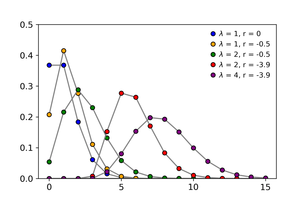
Although the Poisson distribution is most commonly introduced in the context of events accumulating over a fixed time interval, its reach extends well beyond one-dimensional temporal counting. The same mathematical structure applies to the number of events occurring within a given area or volume, effectively generalizing the model to higher spatial dimensions. This makes it a natural tool for describing the locations of random points in space, whether those points represent imperfections embedded in a three-dimensional material, the positions of trees scattered across a two-dimensional forest floor, or the impact sites of asteroids on a planetary surface. The distribution also occupies a distinguished place among discrete-stable distributions, a class of probability laws that retain their form under certain aggregation operations. This stability property, combined with the model's applicability to rare-event systems where many independent opportunities exist, gives the Poisson distribution a foundational role in both theoretical probability and applied statistical modeling across physics, engineering, and the social sciences.
Gallery
Frequently Asked Questions
Who is Poisson distribution?
A discrete probability distribution named after French mathematician Siméon Denis Poisson, it models how many times an event fires off within a fixed window of time or space. Think of it as the go-to character whenever you need to count rare, independent occurrences.
What are Poisson distribution's powers/role?
Its signature move is computing the probability of exactly k events given a known average rate λ, under the assumption that events don't influence one another. It shows up constantly in call-center arrival counts, radioactive decay tallies, and website-hit-per-minute estimates.
How does Poisson distribution's story end?
Its arc wraps up the moment its core assumptions break down—events must stay independent, the rate must remain constant, and only whole-number counts are valid. If any of those conditions fail, a different distribution steps in to carry the narrative.
Why is Poisson distribution important?
It offers a clean, single-parameter model for rare-event counting that underpins queueing theory, reliability engineering, and much of applied probability. Its tidy mathematical form also makes it a natural building block for more elaborate constructs like compound Poisson processes.
What's Poisson distribution's biggest weakness?
Because it locks variance equal to the mean, it struggles with overdispersed data where variability outpaces the average rate. In those situations, fans typically reach for the negative binomial distribution as a more flexible stand-in.
More in Probability & Statistics 1-24
Spotted an error? Know more?
This is a living reference — every entry is fact-audited, and reader corrections feed straight into our audit queue. Suggest an edit · See this site's audit record