
Multivariate normal distribution
Generalization of normal distribution to multiple dimensions.

MartinThoma · CC0
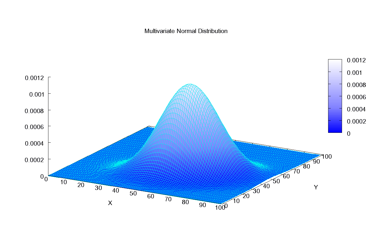
The multivariate normal distribution, also called the multivariate Gaussian or joint normal distribution, extends the one-dimensional normal distribution into higher dimensions. A random vector is considered k-variate normally distributed if every linear combination of its k components follows a univariate normal distribution. Its significance largely comes from the multivariate central limit theorem, and it is commonly used to approximate any set of correlated real-valued random variables, each centered around a mean. A k-dimensional random vector can be expressed with a mean vector μ and a covariance matrix Σ, where Σ is symmetric and positive semidefinite. The inverse of Σ is the precision matrix. A standard normal random vector has independent components, each with zero mean and unit variance. A centered normal random vector is one that can be written as A Z, where Z is a standard normal vector and A is a matrix. More generally, a normal random vector X can be written as μ + A Z, with covariance Σ = A Aᵀ. If Σ is singular, the distribution is degenerate and lacks a density with respect to k-dimensional Lebesgue measure; this occurs, for instance, in the distribution of residuals from ordinary least squares regression. The components of X are generally not independent but result from applying A to independent Gaussian variables. Equivalent definitions include: every linear combination of its components is normally distributed (with zero variance allowed as a point mass), or there exists a vector μ and a symmetric positive semidefinite matrix Σ such that the characteristic function is φ(t) = exp(i tᵀμ - ½ tᵀΣ t). The spherical normal distribution is uniquely characterized by having independent components in any orthogonal coordinate system. When Σ is positive definite, the distribution is non-degenerate and has a density: f(x) = (2π)⁻ᵏ/² |Σ|⁻¹/² exp(-½ (x-μ)ᵀ Σ⁻¹ (x-μ)), where |Σ| is the determinant (generalized variance).
- field
- Probability theory and statistics
- known_for
- Generalization of the univariate normal distribution to higher dimensions; defined such that every linear combination of components has a univariate normal distribution
Lore & Background
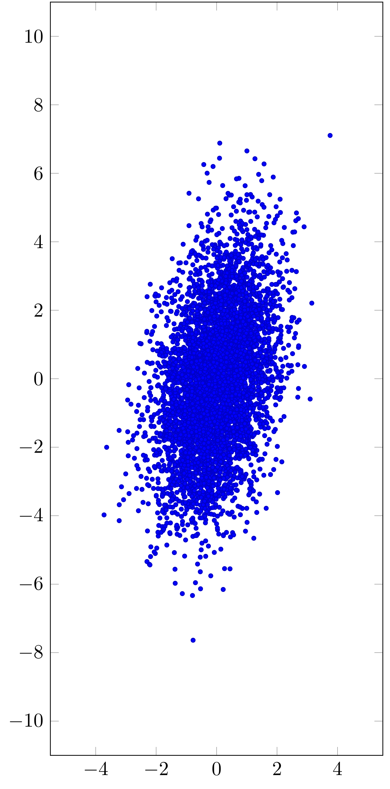
The multivariate normal distribution generalizes the univariate normal distribution to higher dimensions. A random vector is said to follow this distribution if every possible linear combination of its components is itself normally distributed. It is typically denoted as **X ~ N(μ, Σ)** or **X ~ N_k(μ, Σ)**, where **μ** is a k-dimensional mean vector and **Σ** is a k×k covariance matrix, which must be symmetric and positive semidefinite. The inverse of the covariance matrix is known as the precision matrix. In the standard case, all components are independent, each with zero mean and unit variance. A centered normal random vector can be obtained by applying a matrix to such a standard normal vector, while a general normal random vector adds a mean vector to this transformation. When the covariance matrix is positive definite (non-degenerate), the distribution has a probability density function. This density involves the Mahalanobis distance, which measures the distance of a point from the mean. The iso-density contours are ellipses (or higher-dimensional ellipsoids), making the multivariate normal a special case of elliptical distributions. In the bivariate case, the correlation between the two variables determines the orientation and shape of these elliptical contours. If the covariance matrix is singular (degenerate), the distribution does not have a density with respect to standard Lebesgue measure, a situation common in statistics, such as with residual vectors from ordinary least squares regression. The distribution’s importance stems largely from the multivariate central limit theorem, and it is frequently used to approximately model sets of correlated real-valued random variables that cluster around a mean.
Reader's Guide
A standard normal random vector has independent components, each with zero mean and unit variance. A centered normal random vector can be expressed as A Z, where Z is a standard normal random vector and A is a matrix. A normal random vector can be written as X = A Z + μ. In the degenerate case where the covariance matrix is singular, the corresponding distribution has no density; this case arises frequently in statistics, for example in the distribution of the vector of residuals in ordinary least squares regression. The behavior of the multivariate normal distribution is defined by its mean vector and covariance matrix, which together determine the shape and orientation of its probability density. In the non-degenerate case, where the covariance matrix is positive definite, the distribution has a density function that involves the determinant of the covariance matrix and the Mahalanobis distance, a measure of how far a point is from the mean. The iso-density contours of this distribution are ellipses or their higher-dimensional generalizations, making it a special case of elliptical distributions. In the bivariate case, these contours are ellipses whose principal axes align with the eigenvectors of the covariance matrix, and the correlation parameter influences how tightly the distribution clusters along a line. Ecologically and statistically, the multivariate normal distribution is significant because it describes correlated real-valued random variables that cluster around a mean, and its importance stems largely from the multivariate central limit theorem, which justifies its use as an approximate model for many real-world phenomena. The distribution also relates to the concept of a spherical normal distribution, which is uniquely characterized by having independent components in any orthogonal coordinate system.
Did You Know?
- The multivariate normal distribution is a generalization of the one-dimensional normal distribution to higher dimensions.
- A random vector is k-variate normally distributed if every linear combination of its k components has a univariate normal distribution.
- The inverse of the covariance matrix is called the precision matrix.
- In the degenerate case where the covariance matrix is singular, the corresponding distribution has no density.
From One Dimension to Many
The multivariate normal distribution represents a natural extension of the familiar bell curve into higher-dimensional space. Where the univariate normal describes a single random variable centered on a mean with a given spread, its multivariate counterpart captures the joint behavior of k real-valued random variables simultaneously. A particularly elegant characterization holds: a random vector is k-variate normally distributed precisely when every possible linear combination of its components yields a univariate normal result. This property makes the definition both powerful and verifiable, since checking all linear combinations guarantees the full multivariate structure. The distribution's prominence in probability theory and statistics is largely anchored in the multivariate central limit theorem, which ensures that sums of many independent random vectors converge toward this form regardless of the original distributions. In practice, the multivariate normal serves as a flexible approximate model for any collection of possibly correlated variables, each tending to cluster around its own mean value.
The Architecture of Parameters
Every multivariate normal distribution is fully specified by two objects: a mean vector and a covariance matrix. The mean vector μ, of dimension k, collects the expected value of each component, so its i-th entry is simply E[X_i]. The covariance matrix Σ is a k by k symmetric array whose (i, j) entry records the expected product of deviations (X_i − μ_i)(X_j − μ_j), equivalently the covariance between the i-th and j-th components. Together these two parameters encode both the central location and the shape of the distribution in k-dimensional space. A useful derived quantity is the precision matrix Q, defined as the inverse of Σ. This inverse plays a central role in computational statistics and Bayesian inference, where it often appears more naturally than the covariance itself. The standard notation X ~ N(μ, Σ) or, when dimension must be explicit, X ~ N_k(μ, Σ), keeps the parameterization compact. Because the covariance matrix captures all pairwise relationships among the k variables, a single k by k matrix suffices to describe the entire dependence structure, making the parametrization remarkably economical for high-dimensional problems.
Standard and Centered Building Blocks
Two special cases of the multivariate normal serve as foundational building blocks. The standard normal random vector is the simplest: every component is an independent draw from a zero-mean, unit-variance normal distribution, meaning each X_i follows N(0, 1) for i = 1 through k. Because independence forces the covariance matrix to be the identity, the standard normal vector carries no information about correlation and acts as a canonical reference point from which all other multivariate normals can be generated through affine transformations. The centered normal random vector generalizes this idea by requiring the existence of a k by ℓ matrix A such that the vector can be expressed as a linear transformation of a standard normal vector. This construction allows the components to be correlated while preserving the zero-mean property, and the rank of A controls the effective dimensionality of the resulting distribution. Together, these two special cases provide the structural vocabulary from which the full family of multivariate normal distributions is assembled, and they underpin much of the theoretical machinery used in multivariate statistical analysis.
Why It Dominates Statistical Practice
The multivariate normal distribution occupies a position of unusual centrality in probability and statistics, and its dominance rests on a single deep result: the multivariate central limit theorem. This theorem guarantees that when many independent random vectors are summed, the resulting distribution converges to a multivariate normal regardless of the individual distributions of the summands. This universality explains why the multivariate normal appears so frequently as a working model: it is not merely a convenient choice but a mathematically inevitable limit. Beyond this theoretical guarantee, the distribution is practically invaluable because it can approximate, at least roughly, any collection of possibly correlated real-valued random variables, provided each one clusters around a finite mean. The linear-combination definition further ensures that projections of the data onto any direction remain normally distributed, which simplifies hypothesis testing, confidence regions, and regression analysis. In applied fields ranging from engineering to finance, this combination of theoretical justification and computational tractability makes the multivariate normal the default starting point for modeling multivariate uncertainty.
Gallery
Frequently Asked Questions
Who is Multivariate normal distribution?
It is the high-dimensional cousin of the familiar bell curve, extending the one-variable Gaussian into any number of correlated dimensions. Also called the joint normal or multivariate Gaussian, it is defined by the rule that every possible linear combination of its components still follows a standard one-dimensional normal.
What are Multivariate normal distribution's powers/role?
Its core superpower is that any linear combination of its random variables yields a univariate normal, making it the natural home for correlated Gaussian data. In practice it serves as the default model for collections of real-valued variables that each cluster around a mean while being linked to one another.
How does Multivariate normal distribution's story end?
It has no real ending—it is a permanent foundational building block underpinning models in finance, machine learning, and signal processing. Its narrative simply continues through every theorem, simulation, and Bayesian posterior that relies on correlated Gaussian assumptions.
Why is Multivariate normal distribution important?
Its central claim to fame is the multivariate central limit theorem, which guarantees that sums of independent random vectors converge to this distribution regardless of the original shapes. That universality makes it the go-to approximation for correlated real-world measurements across virtually every quantitative field.
What's Multivariate normal distribution's origin story?
It emerged as the natural multi-dimensional extension of the one-variable normal, filling the gap when statisticians needed to model several interdependent quantities simultaneously. The defining rule—every linear projection must be univariate normal—gives it a clean, coordinate-free identity within probability theory.
More in Probability & Statistics 1-24
Spotted an error? Know more?
This is a living reference — every entry is fact-audited, and reader corrections feed straight into our audit queue. Suggest an edit · See this site's audit record