
Normal distribution
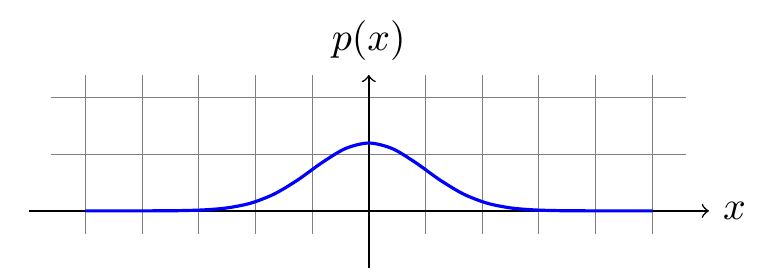
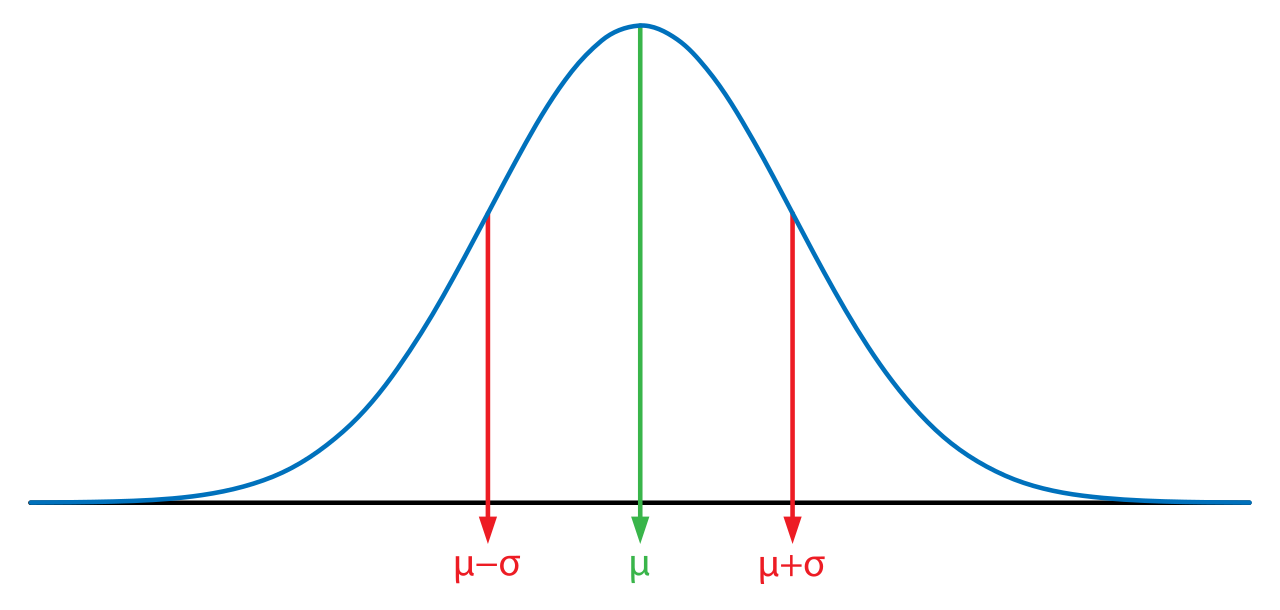
A continuous probability distribution with a bell-shaped density curve.

TYalaA · CC BY-SA 4.0
In probability theory and statistics, the normal distribution—also called the Gaussian distribution—is a continuous probability distribution for real-valued random variables. Its probability density function is defined by two parameters: μ (the mean, which also serves as the median and mode) and σ² (the variance). The standard deviation is the positive square root of the variance, σ. A random variable following this distribution is said to be normally distributed and is known as a normal deviate. These distributions are widely used in statistics, particularly in the natural and social sciences, to model real-valued random variables when the actual distribution is unknown. Their significance largely stems from the central limit theorem, which states that the average of many statistically independent samples from a random variable with finite mean and variance converges to a normal distribution as the sample size grows. As a result, physical quantities that are sums of many independent processes—such as measurement errors—often approximate a normal distribution. Gaussian distributions also have unique properties valuable for analytical work. For example, any linear combination of independent normal deviates is itself a normal deviate. Many methods, including propagation of uncertainty and least squares parameter fitting, can be expressed analytically in explicit form when the relevant variables are normally distributed. However, normal distributions are frequently misapplied in cases where the data are not actually normal, making the model a poor fit. Informally, the normal distribution is sometimes called a bell curve, though many other distributions—such as the Cauchy, Student's t, and logistic—are also bell-shaped. The univariate distribution generalizes to the multivariate normal distribution for vectors and the matrix normal distribution for matrices. **Standard normal distribution** The simplest case is the standard normal distribution (or unit normal distribution), where μ = 0 and σ² = 1. Its probability density function is φ(z).
- field
- Probability theory and statistics
- known_for
- Bell-shaped curve, central limit theorem, linear combination of independent normal deviates
Lore & Background
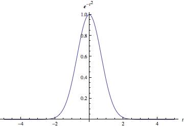
The simplest case of a normal distribution is the standard normal distribution, with μ = 0 and σ² = 1. Its density function φ(z) = e^{-z²/2} / √(2π) has its peak at z = 0 and inflection points at z = +1 and z = -1. Some authors have used different definitions; for instance, Carl Friedrich Gauss used the form φ(z) = (1/√π) e^{-z²} (which has a variance of 1/2) in his work, though he did not define a 'standard normal' in the modern sense. Similarly, Stephen Stigler has noted the historical appearance of the form φ(z) = e^{-π z²} (which has a variance of 1/(2π)), but he did not define the standard normal in that way.
Reader's Guide
A normal distribution is sometimes informally called a bell curve, though many other distributions are bell-shaped. Its importance stems from the central limit theorem, which states that the average of many independent samples of a random variable with finite mean and variance converges to a normal distribution as the number of samples increases. Physical quantities that are the sum of many independent processes, such as measurement errors, often have nearly normal distributions. Gaussian distributions have unique properties: any linear combination of independent normal deviates is a normal deviate, and many methods like propagation of uncertainty and least squares parameter fitting can be derived analytically when variables are normally distributed. However, normal distributions are frequently misused in contexts where the assumption of normality is not met. The univariate distribution is generalized for vectors in the multivariate normal distribution and for matrices in the matrix normal distribution.
Did You Know?
- The standard normal distribution has mean 0 and variance 1.
- Carl Friedrich Gauss used the form φ(z) = (1/√π) e^{-z²} in his work, which has a variance of 1/2, though he did not define a 'standard normal' in the modern sense.
- Stephen Stigler noted the historical appearance of the form φ(z) = e^{-π z²}, which has a variance of 1/(2π), but he did not define the standard normal in that way.
- Any linear combination of a fixed collection of independent normal deviates is a normal deviate.
The Mathematical Architecture of the Gaussian Curve
The normal distribution is a continuous probability model defined over all real numbers, governed by just two parameters. The first, μ (mu), simultaneously serves as the mean, median, and mode of the distribution, anchoring the curve's center. The second, σ² (sigma-squared), represents the variance, while its positive square root σ gives the standard deviation, controlling how broadly the probability mass spreads. Together they produce the familiar density function: a prefactor of one over the square root of two pi sigma-squared, multiplied by the exponential of negative (x minus mu) squared over two sigma-squared. The simplest incarnation, the standard normal, sets both parameters to their most neutral values—mean zero and variance one. Its density peaks at exactly one over the square root of two pi when z equals zero, and it bends at the inflection points z equals plus or minus one. Interestingly, the very definition of "standard" has varied across eras: Gauss once chose a version with variance one-half, while the statistician Stephen Stigler proposed yet another variant with a different scaling constant.
The Central Limit Theorem and Ubiquity
The normal distribution's dominance in statistics owes much to the central limit theorem, which guarantees that when you average a large collection of statistically independent observations drawn from any distribution possessing a finite mean and variance, the resulting average converges toward a normal shape as the sample count grows. This single principle explains why physical quantities that accumulate through many independent small effects—measurement errors being a classic example—tend to look approximately Gaussian even when the underlying individual contributions are far from normal. Because of this convergence property, researchers across the natural and social sciences routinely reach for the normal model as a working assumption whenever the true distribution of a real-valued random variable remains unknown. It becomes a default lens through which uncertainty is quantified, predictions are framed, and statistical tests are constructed, making the normal distribution arguably the single most invoked probability model in applied science.
Analytic Elegance and Practical Tools
Beyond its empirical prevalence, the Gaussian distribution possesses algebraic properties that make it extraordinarily tractable in mathematical work. A standout feature is closure under linear combination: if you take any fixed set of independent normal deviates and form a weighted sum, the result is itself a normal deviate. This closure property cascades into a wide range of analytic results. Propagation of uncertainty—the task of tracking how measurement errors in input variables flow through a computation to affect an output—yields clean, explicit formulas when the inputs are Gaussian. Similarly, least-squares parameter fitting, a cornerstone of regression analysis, admits closed-form solutions under normality assumptions. These analytic conveniences mean that researchers can derive exact expressions rather than resort to numerical approximations, giving the normal distribution a dual role: it is both a descriptive model of real-world data and a computational workhorse that keeps the mathematics of statistical inference manageable.
Misuse, Misnaming, and Generalizations
Despite its popularity, the normal distribution is frequently deployed in settings where its assumptions simply do not hold, leading to misleading conclusions when the data are a poor fit for the Gaussian model. The colloquial label "bell curve" compounds the confusion, because many other distributions—including the Cauchy, Student's t, and logistic distributions—also exhibit a bell-shaped silhouette, yet differ fundamentally in their tails, symmetry, or parameter structure. The term "standard normal" itself has not been immune to ambiguity, as different authors have historically attached it to variants with different variances. On the constructive side, the univariate framework extends naturally: vectors of jointly normal random variables give rise to the multivariate normal distribution, and the concept reaches further still into the matrix normal distribution, where the random object is an entire matrix rather than a single scalar. These generalizations preserve the Gaussian character while accommodating the multidimensional structure common in modern data analysis.
Gallery
Frequently Asked Questions
Who is Normal distribution?
The Normal distribution (a.k.a. Gaussian) is a continuous probability model for real-valued random variables, fully specified by just two numbers: a center μ and a spread σ². It is the distribution that gives us the famous symmetric bell-shaped density curve.
What are Normal distribution's powers/role?
Its most celebrated ability is closure: any linear combination of independent normal random variables is itself normal, so it behaves beautifully under algebraic manipulation. It also acts as the default stand-in whenever a real-valued variable's true distribution is unknown.
How does Normal distribution's story end?
It never truly ends—the density curve approaches the horizontal axis asymptotically on both sides without ever touching it. In other words, every point on the real line carries some nonzero density, no matter how far out in the tails you look.
Why is Normal distribution important?
The Central Limit Theorem tells us that averages of many independent observations converge toward a normal shape, which explains why the bell curve shows up across natural and social sciences. This universality is the main reason statisticians reach for it as a first approximation.
What are Normal distribution's key stats?
Two parameters do all the work: μ simultaneously fixes the mean, median, and mode (the peak of the bell), while σ² governs how wide or narrow the curve is. Swap either value and you get a brand-new normal distribution.
More in Probability & Statistics 1-24
Spotted an error? Know more?
This is a living reference — every entry is fact-audited, and reader corrections feed straight into our audit queue. Suggest an edit · See this site's audit record