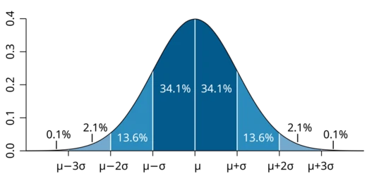
Probability density function

A probability density function (PDF), also called a density function or simply the density of an absolutely continuous random variable, describes how probability is distributed across the possible values that variable can take. At any specific point in the sample space, the PDF gives a "relative probability"—it indicates how likely it is that the random variable will be near that point compared to another, even though the exact probability of hitting any single value is zero. In essence, probability density is the probability per unit of measurement.

Rather than assigning probability to individual values, the PDF is used to find the probability that the random variable falls within a given range. This probability equals the integral (the area under the curve) of the PDF between the lower and upper bounds of that range. The PDF is always nonnegative, and the total area under the entire curve equals one, meaning there is a 100% chance the variable takes some value within its possible set.

The terms "probability distribution function" and "probability function" are sometimes used interchangeably with PDF, but this is not standard among probabilists and statisticians. In other contexts, "probability distribution function" might refer to the cumulative distribution function (CDF), a probability mass function (PMF), or a function defined over general sets. The word "density" itself can also be applied to the PMF, causing confusion. Generally, the PMF is used for discrete random variables (those taking values from a countable set), while the PDF is used for continuous ones. Both are essential in statistical inference.

**Example** Consider bacteria that typically live between 20 and 30 hours. The probability that a bacterium lives exactly 5 hours is zero—this is about an idealized continuous variable, not a recorded observation. Many bacteria live about 5 hours, but none die at precisely 5.000... hours. However, the chance of dying between 5 and 5.01 hours is quantifiable; suppose it is 0.02 (2%). Then the chance of dying between 5 and 5.001 hours is about 0.002, one-tenth as long. Similarly, between 5 and 5.0001 hours, it is about 0.0002.

Here, the ratio (probability of dying during an interval) divided by (interval length) is roughly constant at 2 per hour. For the 0.01-hour interval from 5 to 5.01 hours, that ratio is 0.02 / 0.01 = 2 hour⁻¹. This value, 2 hour⁻¹, is the probability density at around 5 hours. So the probability of dying at exactly 5 hours can be written as (2 hour⁻¹) dt, where dt is an infinitesimally small time window. For instance, the chance of dying between 5 hours and 5 hours plus one nanosecond is (2 hour⁻¹) × (1 nanosecond). A PDF f exists such that f(5 hours) = 2 hour⁻¹, and the integral of f over any time window gives the probability of death in that window.

**Absolutely continuous univariate distributions** A PDF is most often tied to absolutely continuous univariate distributions. A random variable X has density f, a nonnegative Lebesgue-integrable function, if: - For any real numbers a and b, P(a ≤ X ≤ b) = ∫ₐᵇ f(x) dx. If F is the cumulative distribution function of X, then F(x) = ∫₋∞ˣ f(t) dt, and where F is differentiable, f(x) = F'(x). Intuitively, f(x) dx approximates the probability that X falls in the infinitesimal interval [x, x+dx].

**Formal definition** (This definition can be extended using measure-theoretic probability.) A random variable X with values in a measurable space (often ℝ with Borel sets) has a probability distribution given by the pushforward measure X∗P. The density f of X with respect to a reference measure μ on the space is the Radon–Nikodym derivative: f = d(X∗P)/dμ. That is, f is any measurable function such that for any measurable set A, P(X ∈ A) = ∫ₐ f dμ.

**Discussion** In the continuous univariate case, the reference measure is Lebesgue measure. For a discrete random variable, the probability mass function is the density with respect to counting measure on the sample space (e.g., integers). A density cannot be defined with respect to an arbitrary measure (e.g., counting measure cannot serve as a reference for a continuous variable). When a density exists, it is almost unique—any two such densities agree almost everywhere.

**Further details** Unlike a probability, a PDF can exceed one. For example, the continuous uniform distribution over a short interval has a density greater than one.