Air quality modeling

Atmospheric layers

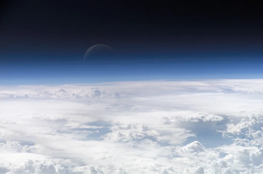
The Earth's atmosphere is divided into layers that influence where airborne pollutants disperse. The lowest layer, the troposphere, extends from sea-level to about 18 km and contains roughly 80 percent of the atmosphere's mass. Above it lies the stratosphere (18 km to about 50 km), then the mesosphere (50 km to about 80 km). Layers above 80 km are insignificant for dispersion modeling.

Within the troposphere, the lowest portion is the planetary boundary layer (PBL), also called the atmospheric boundary layer. In the PBL, air temperature decreases with altitude until reaching a capping inversion, where warmer air sits above cooler air. The region below this inversion is the convective planetary boundary layer, typically 1.5 to 2 km in height. Above the inversion lies the free troposphere, extending to the tropopause.

In tropical and mid-latitudes during daytime, the free convective layer can span the entire troposphere, up to 10 to 18 km in the Intertropical Convergence Zone. The PBL is critical for pollutant transport because turbulent wind dynamics are strongest near the Earth's surface. The part of the PBL between the surface and the inversion base is called the mixing layer; almost all emitted airborne pollutants are transported and dispersed within it. Some emissions penetrate the inversion and enter the free troposphere.

Many atmospheric dispersion models are boundary layer models, focusing on dispersion within the PBL. Mesoscale models, despite their name, extend horizontally up to a few hundred kilometers and do not model dispersion in the mesosphere.

Gaussian air pollutant dispersion equation

The technical literature on air pollution dispersion dates back to the 1930s. An early plume dispersion equation by Bosanquet and Pearson did not assume a Gaussian distribution nor include ground reflection. In 1947, Sir Graham Sutton derived an equation that assumed Gaussian distribution for vertical and crosswind dispersion and included ground reflection. Between the late 1960s and today, stringent environmental regulations spurred the development of many computer programs called air dispersion models.

Most of these models are based on the complete equation for Gaussian dispersion modeling of continuous, buoyant plumes. That equation includes upward reflection from the ground and downward reflection from any inversion lid. The sum of its four exponential terms converges rapidly; for most cases, summation with m = 1, 2, and 3 provides an adequate solution. The dispersion parameters σy and σz are functions of atmospheric stability class and downwind distance.

The two most important variables affecting dispersion are the height of the emission source and the degree of atmospheric turbulence. Equations for σy and σz take the form exp(I + J ln(x) + K [ln(x)]^2), with units in meters. Stability classes, proposed by F. Pasquill, range from A (extremely unstable) through D (neutral) to F (moderately stable).

Briggs plume rise equations

The Gaussian dispersion equation requires the plume centerline height H, which is the sum of the physical stack height Hs and the plume rise ΔH due to buoyancy. To determine ΔH, many air dispersion models developed between the late 1960s and early 2000s used the Briggs equations. G.A. Briggs first published plume rise observations and comparisons in 1965. In 1968, at a symposium sponsored by CONCAWE, he compared many existing plume rise models.

That same year, Briggs wrote a section in a publication edited by Slade on comparative analyses of plume rise models. In 1969, he published a critical review proposing a set of equations that became known as the Briggs equations, which he later modified in 1971 and 1972. Briggs divided plumes into four categories: cold jet plumes in calm air, cold jet plumes in windy air, hot buoyant plumes in calm air, and hot buoyant plumes in windy air. He considered cold jet plumes dominated by initial velocity momentum and hot buoyant plumes dominated by buoyant momentum.

The widely used Briggs equations are those for bent-over, hot buoyant plumes, based on observations from typical combustion sources such as flue gas stacks of steam-generating boilers in large power plants. Stack exit velocities in those observations were likely 20 to 100 ft/s (6 to 30 m/s) with exit temperatures of 250 to 500 °F (120 to 260 °C). A logic diagram for using the Briggs equations for bent-over buoyant plumes exists, and the parameters are discussed in Beychok's book.